
In this third and final installment in the series, we will discuss how to detect interactions and share code and tools we built at Vista to address this issue. This post will necessarily be a little more technical than the previous ones because detection relies on statistical methods. However, we have attempted to keep the explanations easy to follow, even for those unfamiliar with the statistical concepts and techniques used.
Theoretical Background
Testing for interactions is a form of hypothesis testing, very similar to regular A/B testing. The null hypothesis that we will try to reject states that two experiments are not interacting. If the data are improbable under that hypothesis (i.e., we find a low p-value), then we can reject this null hypothesis and claim that there is an interaction.
As with regular hypothesis testing, different statistical methods are available to test this absence of interactions hypothesis. In this post, we will describe our approach, although we acknowledge that there are probably many other equally valid alternatives. There’s more than one way to cook an egg; what follows is simply how we choose to cook ours. If you cook yours differently, please publish your approach and share it with us.
Testing for Traffic Interactions
The first hypothesis we want to test is whether there is evidence for the presence of traffic interactions. We want to know if traffic distribution in one experiment is affected by another experiment. For this, we can use a Chi-squared test to test for statistical independence. This same test is also used for detecting Sample Ratio Mismatch (SRM). The main difference is that in the case of interactions, we have two experiments instead of one. Instead of comparing actual observed traffic with theoretically expected traffic as we would in the sample ratio mismatch test, we will use a contingency table that contains counts for every combination of treatment statuses of both experiments.
For two basic A/B tests, the input data will look something like this:
| Users in A of Experiment 1 | Users in B of Experiment 1 | |
|---|---|---|
| Users in A of Experiment 2 | 257 | 270 |
| Users in B of Experiment 2 | 239 | 234 |
Using R to generate some data and run the Chi-squared test, the output will look something like this:
> set.seed(42)
> df = data.frame(x1 = rbinom(n=1000, size=1, prob=0.5), x2 = rbinom(n=1000, size=1, prob=0.5))
> t = table(df)
> chisq.test(t)

Pearson's Chi-squared test with Yates' continuity correction

data:  t
X-squared = 0.24309, df = 1, p-value = 0.622
As explained above, we are interested in the p-value. In this example, the p-value of 0.622 is greater than our threshold, commonly 0.05, and thus we can conclude—in this case correctly—that there is no evidence for a traffic interaction.
Testing for Metric Interactions
The second hypothesis we want to test is whether there is evidence for the presence of metric interactions. However, in theory, we could use the same Chi-squared test as above to test for statistical independence in the case of the binomial (yes/no) metrics. We would do so by using counts of conversions rather than counts of visitors in each cell. A more powerful and flexible method is to use a regression.
Using a regression will allow us to estimate the relationships between a dependent variable (in our case, a metric) and one or more independent variables (in our case, the treatment statuses). The output of a regression model usually includes significance tests for the existence of those relationships. If we were to apply a regression using only the treatment status of one experiment, we would get a result that is essentially equivalent to the statistical test used in a regular A/B test. In statistical terms, we would write metric_value ~ status, defining a model which tries to estimate the metric value given only the treatment status as input.
Regression models are not limited to using a single independent variable. By including the treatment status of a second experiment as well as a so-called “interaction term” in our regression model, we can get an estimate (and p-value) for the interaction effect (if any) between the two experiments. This approach works for binomial as well as continuous metrics. In statistical terms, we would write metric_value ~ status1*status2, which expands to metric_value ~ status1 + status2 + status1_and_status2 and defines a model which tries to estimate the metric value given both treatment statuses as input as well as a third input that indicates if a user was in both tests at the same time.
For two basic A/B tests, the input data will look like this:
| User | Experiment 1 | Experiment 2 | Metric value |
|---|---|---|---|
| User 1 | A | B | 40,70 |
| User 2 | B | A | 15,60 |
Using R to run a regression on this data frame df, the output will look something like this:
> summary(lm(metric_value ~ exp_1*exp_2, data = df))

Call:
lm(formula = metric_value ~ exp_1 * exp_2, data = df)

Residuals:
   Min     1Q Median     3Q    Max
-25.38 -22.34 -20.82 -20.20 280.00

Coefficients:
            Estimate Std. Error t value Pr(>|t|)
(Intercept)  20.1959     0.3081  65.543  < 2e-16 ***
exp_1         0.6201     0.4339   1.429    0.153
exp_2         2.1495     0.4348   4.943 7.69e-07 ***
exp_1:exp_2   2.4183     0.6146   3.935 8.33e-05 ***
---
Signif. codes:  0 ‘***’ 0.001 ‘**’ 0.01 ‘*’ 0.05 ‘.’ 0.1 ‘ ’ 1

Residual standard error: 48.59 on 99996 degrees of freedom
Multiple R-squared:  0.001691,      Adjusted R-squared:  0.001661
F-statistic: 56.45 on 3 and 99996 DF,  p-value: < 2.2e-16
Again, as explained above, we are interested in the p-value. This regression outputs several p-values for different inputs to the model. For our use case, we are interested in the p-value related to the interaction term exp_1:exp_2 on line 15. The example above shows evidence for an interaction because the p-value is very low—8.33e-05.
The simulation code for this approach is included in Appendix A. A Python equivalent for the regression function is included in Appendix B.
Note that this approach requires user-level data—one row per user. From a performance perspective, using a Chi-squared test with less power might be preferable if there are many combinations of experiments to test for metric interactions.
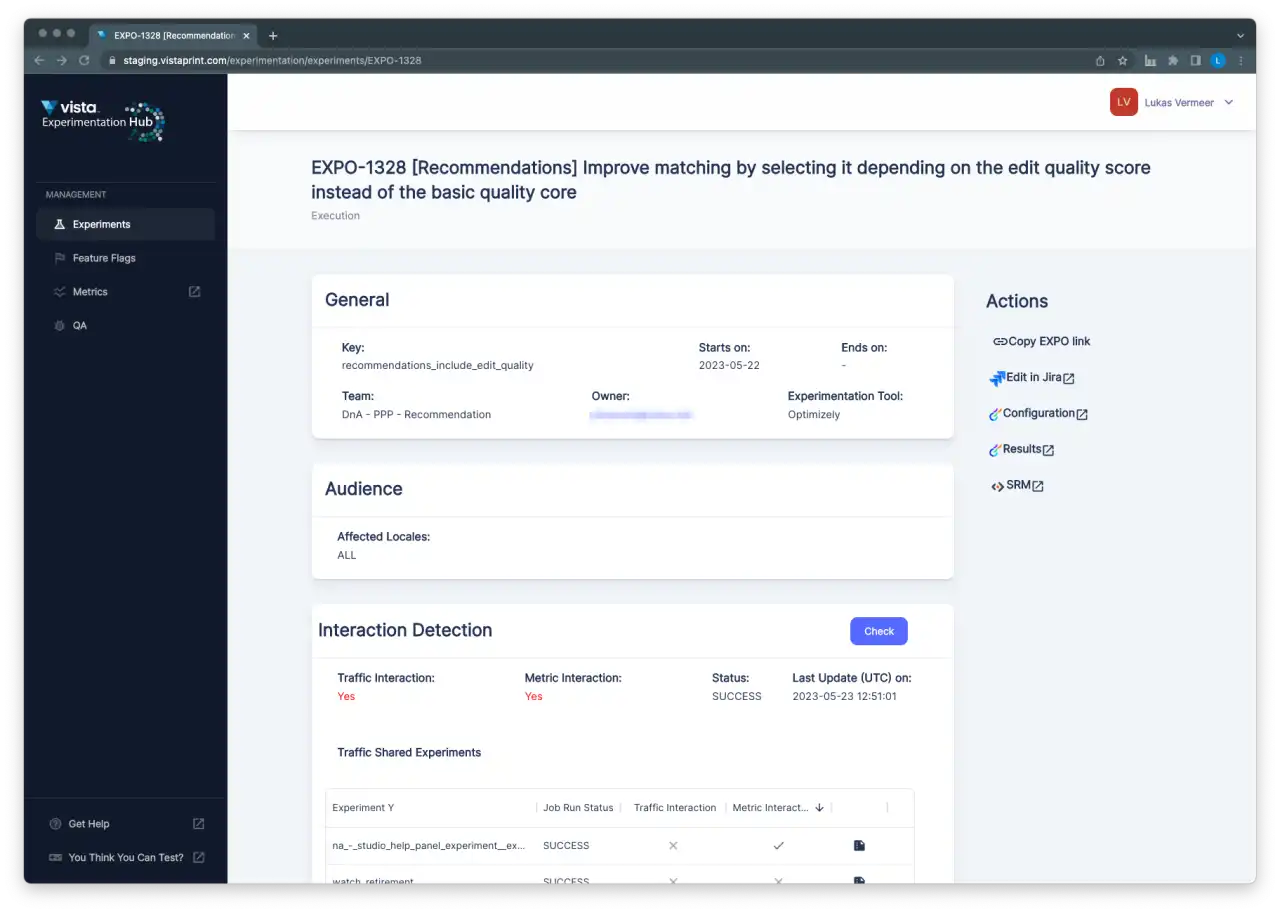
Practical Implementation
At Vista, we want teams to be able to run experiments with very little involvement from our central team or even their embedded analysts. This self-service approach includes data quality checks such as testing for interactions.
We wanted to make these checks available to internal users who might not be familiar with R, Python, or the underlying data. To accomplish this, we initially built two simple dashboards: one to find candidates and one to test for interactions between candidates. Ultimately, we might build additional automation on top of these MVP data products. We are sharing these early iterations to help others in the industry take these first steps.
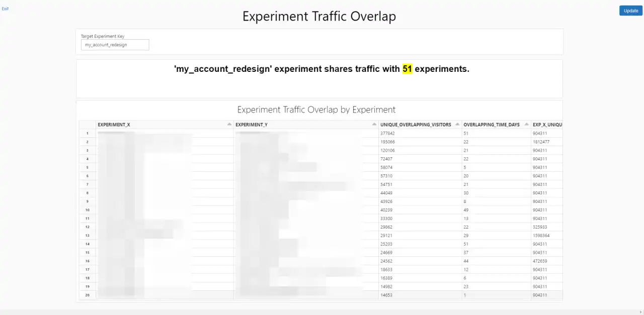
Experiment Traffic Overlap Dashboard
Two experiments can only interact if they share traffic. If zero users are exposed to both experiments, there can be no interaction effects between the two. Because we run experiments in many different locales and on many different subgroups, we needed to give our experimenters a way to identify experiments that share traffic with theirs first.
The Experiment Traffic Overlap dashboard uses a simple join query to generate a list of experiments that share traffic with a given user input, experiment. The dashboard also includes information about how many users and runtime days overlap compared to each experiment’s overall traffic and runtime in isolation. If the overlap is relatively small compared to traffic in general, the potential impact of interactions will be diminished. This overlap helps experimenters quickly identify experiments that are likely candidates to check for interactions with.
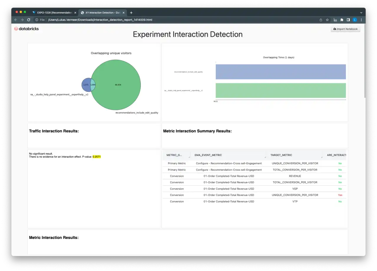
Experiment Interaction Detection Dashboard
Once two experiments to test for interactions have been identified, the second dashboard helps users perform all the necessary tests and provides visual indications of the amount of overlap between the two experiments. The dashboard includes a summary of the results, as well as the detailed output of the Chi-squared test and regression models for power users.
Future Work
Industry experience suggests that interaction effects are relatively rare in practice. We wanted to make sure we have the capability to test whether this is also the case for Vista without unduly investing resources in what might be a relatively rare risk. The first iterations of the dashboards were created as standalone applications to allow for more rapid prototyping and development. We were interested to start collecting real-world examples of interacting experiments as quickly as possible.
Now that we have the basic functionality and initial user feedback, we will need to decide whether we want to invest further in this capability. So far, we have not encountered any examples of interactions, and we will continue to monitor manually with the tooling we have built. If we do, at some point, decide to invest further, we will likely integrate more tightly with the main workflows and tools that our experimenters use to increase awareness and adoption. This integration would require us to spend time making our solutions more scalable, as we expect increased integration will result in increased usage of these reports.
Conclusion
In this series, we have defined two kinds of interaction effects and their potential consequences, discussed possible strategies for avoiding and detecting interactions, and shared some of our tools and processes to accomplish these things. We hope we have convinced you that complete avoidance of experiment interactions is not always feasible, could be prohibitively costly, and that there are occasionally unexpected benefits to detecting interaction effects. Furthermore, avoiding interactions altogether may not be desirable, and detection mechanisms are relatively easy to implement.
Our recommended strategy thus remains: avoid some and detect others.
Avoid potential functional conflicts before any users are exposed using internal processes and tools to provide teams with more visibility on what other teams are testing. Detect interaction effects when they happen using the statistical techniques explained in this final post in the series.
Appendix A: Simulated examples in R
The following R code will generate data for a simulated interaction effect (or no effect if interaction_effect is set to 0) and then test for the presence of such an effect.
sample_size <- 100000
base_rate <- 0.2
base_rpv <- 100
sd_rpv <- 40
lift <- c(0.05, 0.1)
interaction_effect <- 0.1

# given treatment assignments for a user returns revenue
outcome <- function(u) {
    # if not converted, or revenue <0 return 0
    if (rbinom(n=1, size=1, prob=base_rate) == 0 | u['control_rpv'] <= 0) {
        return(0)
    }

    p = u['control_rpv']

    # if user is in variant of test 1, apply lift 1
    if (u['exp_1']) { p = p * (1+lift[1]) }

    # if user is in variant of test 2, apply lift 2
    if (u['exp_2']) { p = p * (1+lift[2]) }

    # if user is in variant of test 1 and test 2, apply interaction effect
    if (u['exp_1'] && u['exp_2']) { p = p * (1+u['interaction_effect']) }

    # conversion with probability p
    return(p)
}

run <- function(i) {
    # construct data frame with treatment assignments for all users in both tests
    df = data.frame(exp_1 = rbinom(n=sample_size, size=1, prob=0.5),
        exp_2 = rbinom(n=sample_size, size=1, prob=0.5),
        control_rpv = rnorm(n=sample_size, mean=base_rpv, sd=sd_rpv),
        interaction_effect = i)

    # add column for conversion outcome of each user
    df['revenue'] = apply(df, 1, outcome)

    # run regression with interaction term
    s <- summary(lm(revenue ~ exp_1*exp_2, data = df))

    return(s$coefficients['exp_1:exp_2',4])
}

# one run
run(interaction_effect)
Appendix B: Python equivalent to run a regression
The following Python code is equivalent to the R regression example included earlier in this post.
import pandas as pd
from statsmodels.formula.api import ols
model = ols("REVENUE ~ X_VARIATION_NAME * Y_VARIATION_NAME", data=pdf_xy_rpv)
results = model.fit()
results.summary()